Air Quality & Visibility

14.1 General Description¹⁰⁶, ¹⁰⁷

When the Clean Water Act (1977, 1990), Clean Air Act (1970, 1990), and the Endangered Species Act (1973) were introduced and subsequently amended by Congress, the national priority to provide citizens and wildlife with the healthiest environment possible had important implications and ramifications for each state. Besides mandates to better monitor all pollutants, states were directed to conform to new pollution standards as established by the Environmental Protection Agency (EPA).

Figure 14.1

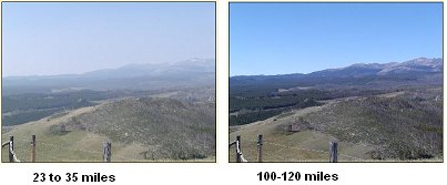
Figure 14.1. Example of Cloud Peak Wilderness Area visibility comparisons

Since then, many states have expressed dissatisfaction with the EPA on several counts. The first is that the federal government limits the amount of funding it provides to states to meet these requirements (unfunded mandates), and secondly, the pollution limits apply equally to all states although each state has unique attributes such as population size, topography, types and amounts of industry, differing agricultural practices, and climate just to name a few. After the 1970s, when researchers began touting global warming (the 1970s was an era when global cooling was in vogue), the issue of increased greenhouse gases became the rallying cry for environmentalists. It has been believed that with increased carbon dioxide (CO₂) emissions, the earth would eventually warm like its sister planet, Venus, whose atmosphere is composed largely of CO₂ and is hotter than the melting point of lead. However, as was discussed in the chapter on climate change, water vapor (H₂O) probably has a greater influence on climate change through its complex positive and negative feedback mechanisms. As the controversy and emotions escalate in the years to come, the bottom line is that, if our quality of life is to be maintained or improved; conservation measures, development of new renewable resources, and retrofitting existing industries to limit pollution are important considerations for everyone.

14.2 Manmade Pollution

Despite the scientific and political issues surrounding pollution, Wyoming continues to have generally good air and water quality. This is due to a low amount of introduced manmade aerosols, low quantity of natural water vapor and airborne particulates, low population, and slow industrial growth. Even on poor visibility days, considerable distances are achieved (Figure 14.1). As shown in Figure 14.2, Sweetwater, Laramie, and Natrona Counties had the highest gross annual tonnage of emissions in 1999 while Hot Springs County had the lowest. "White" depicted counties had no monitoring equipment in 1999. A further breakdown of the 263 industrial plants that emitted pollutants are shown in Figure 14.3. Emission density maps showing Wyoming's various pollutants is depicted in Figure 14.4. Generally, the highest concentration of aerosols and particulates are located over southeast Wyoming with SO₂confined to the southern half of the state. The Scorecard ranks counties by total tons per county rather than considering tons per square mile of a county's total jurisdictional land and water area. The emission gradesheets (Table 14.A.) which are accessible through the website¹¹¹ consider county-by-county air emission densities in tons per square mile of the following pollutants: CO (carbon monoxide), Pb (lead) compounds, NO_x (nitric oxide), VOC (volatile organic compounds), (PM₁₀) particulate matter less than or equal to 10 micrometers, (PM_2.5) particulate matter less than or equal to 2.5 micrometers, NH₃ (ammonia), SO₂ (sulfur dioxide), total HAP (harzardous air pollution), and two particular HAP's, namely diesel emissions and acrolein emissions. The grades are based on emission densities of pollutant tons per square mile.

Figure 14.2

Figure 14.2. Wyoming total emissions by county (amount) and square mile (density) (1999)

Figure 14.3

Figure 14.3. Wyoming emission facilities and pollution monitoring sites¹⁰⁸

Figure 14.4

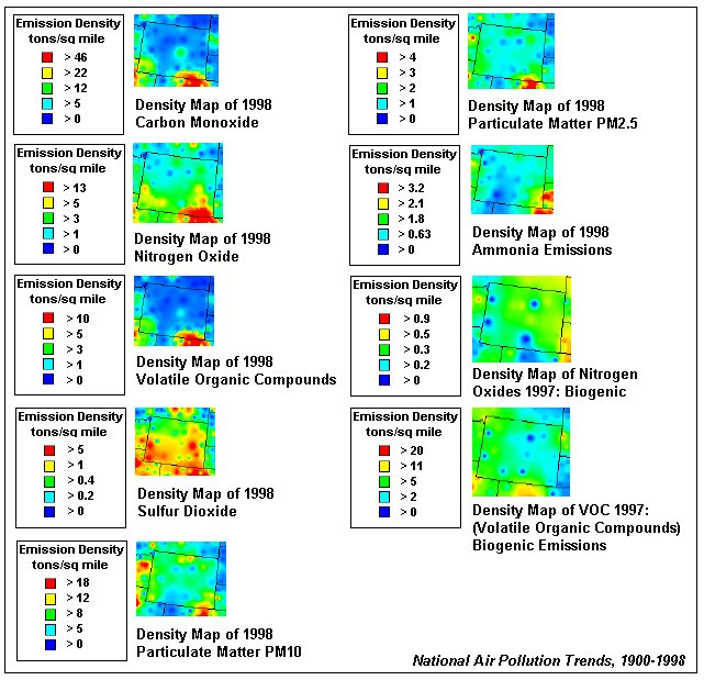
Figure 14.4. Wyoming pollutants as a function of density (1997-1998)

For the first eight pollutants except lead and its compounds, (CO through SO₂, except Pb), emissions are based on 1999 data from the National Emission Trends (NET) section of the EPA's online database AIRData.¹⁰⁹ Lead, total HAP, and acrolein are 1996 data, also from AIRData but under the section National Toxics Inventory (NTI). Diesel emissions are 1996 data from the EPA Air Toxics Website.¹¹⁰ Diesel emissions top the list of air pollutants adding to cancer risk. Acrolein (CH₂CHCHO, pronounced a-kro'-lee-in, "acrid+olein") is the dominant air pollutant for non-cancer hazard. It is an air pollutant produced by forest and wildfires, open burns, structure fires, and as a combustion by-product of gasoline, diesel, and jet engines. One can find related consideration of these pollutants at online references.¹¹¹

The ambient gradesheets (Table 14.B.) reflect 10 EPA standards for air pollutant concentrations. These concentration limits are for various sampling periods from one hour to annually, and for six criteria air pollutants, namely CO, Pb, NO₂, Ozone (O₃), PM, and SO₂. Grade F means exceeding the EPA standard.

Good air quality¹¹² is necessary to avoid harmful health effects. According to the EPA, poor air quality causes visual impairment (Figure 14.5), reduced work capacity, reduced manual dexterity, poor learning ability, difficulty in performing complex tasks, neurological impairments, seizures, mental retardation, behavioral disorders, changes in airway responsiveness, respiratory illness, susceptibility to respiratory infection, lung inflammation, aggravation of respiratory conditions, chest pain, cough, decreased lung function, increased hospital admissions, aggravation of cardiovascular disease, and premature death. See Figure 14.6 for criteria list.

Note that NO₂ levels are usually so low that they pose little direct threat to human health. NO₂ however is a concern because it plays a significant role in the formation of O₃, particle pollution, haze, and acid rain.

Table 14.A.: Wyoming county scorecard: emission gradesheets (1999)

Table 14.A.

Table 14.B.: Wyoming county scorecard: ambient gradesheet (1999)

Table 14.B.

Figure 14.5

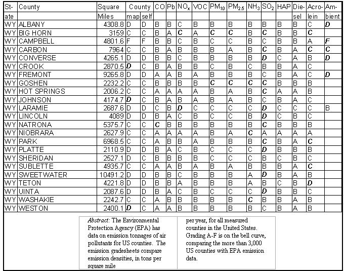
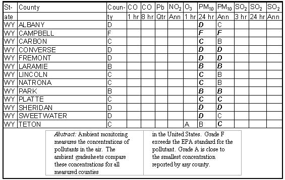
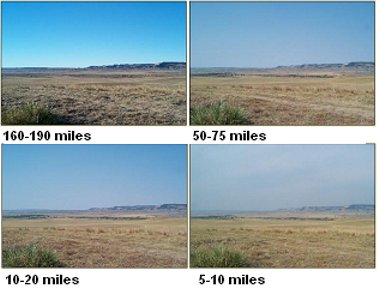
Figure 14.5. Example of Thunder Basin National Grasslands visibility comparisons.

Figure 14.6

Figure 14.6. National Air Quality Index standards

14.3 Natural Pollution¹¹³

Not all pollution is manmade. Because Wyoming is the windiest state in the country, visibility can be frequently and severely limited during times of smoke, haze, and blowing snow, dust^113a, and sand. Besides spoiling a normally pristine mountain view, the radiative effects from dust events may temporarily affect solar electric generating technologies that use collecting cells. Regional forest fires or long range transport of desert dust can trigger temporary losses of beam and daily irradiation in excess of 30 percent.¹¹⁴ Atmospheric aerosol particles influence the earth's radiation balance both directly by scattering and absorbing solar radiation, and indirectly by acting as cloud condensation nuclei (CCN). Increased aerosol and CCN concentrations lead not only to increased scattering of light back to space, but also to higher cloud albedo. Enhanced CCN concentrations can also lead to increased cloud lifetimes and delay or reduce precipitation events.

In Figure 14.7, Figure 14.9, Figure 14.11, and Figure 14.13, horizontal visibilities for Casper, Cheyenne, Lander, and Sheridan reveal that, on average, visibilities are much greater than experienced in the eastern half of the US. Generally, mountains in the distance serve as range markers. As a result, measurements are grouped at specific visibility distances. In Figure 14.8, Figure 14.10, Figure 14.12, and Figure 14.14, the average broadband aerosol optical depth frequencies for Wyoming's four first class weather stations show that in winter, the air is frequently quite clear. Conditions can deteriorate in the summer, although this happens infrequently.

Figure 14.7

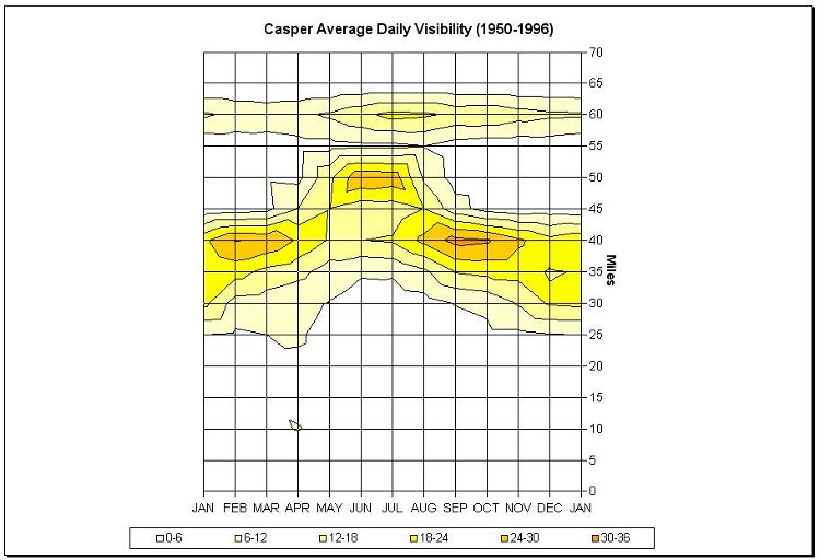
Figure 14.7. Casper horizontal visibility frequency (%) based on hourly observations (1961-1990) (in miles)

Figure 14.8

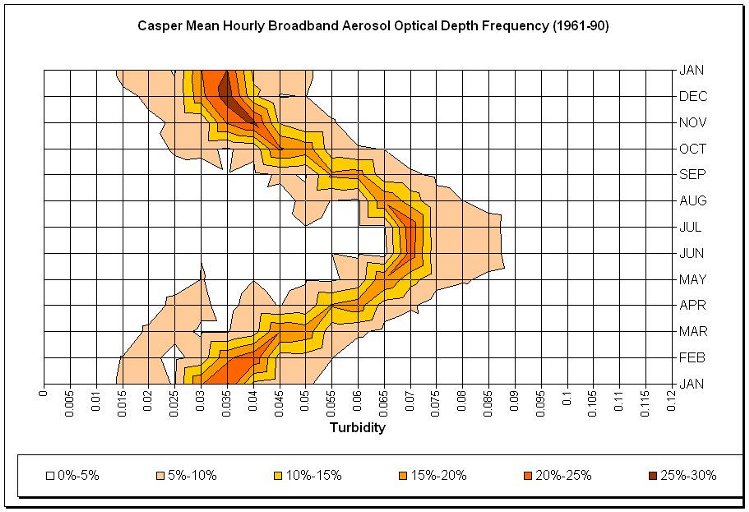
Figure 14.8. Casper broadband aerosol optical depth frequency based on hourly data (1961-90)

Figure 14.9

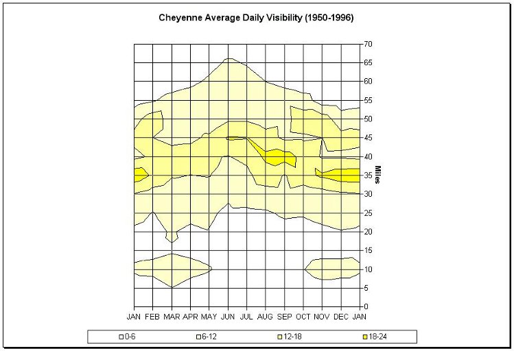
Figure 14.9. Same as Figure 14.7 except for Cheyenne (note different scaling)

Figure 14.10

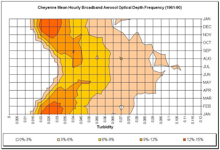
Figure 14.10. Same as Figure 14.8 except for Cheyenne (note different scaling)

Figure 14.11

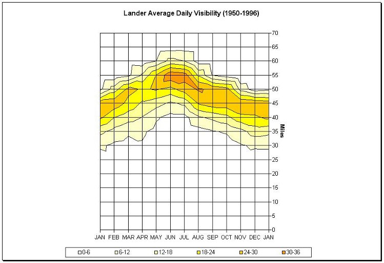
Figure 14.11. Same as Figure 14.7 except for Lander

Figure 14.12

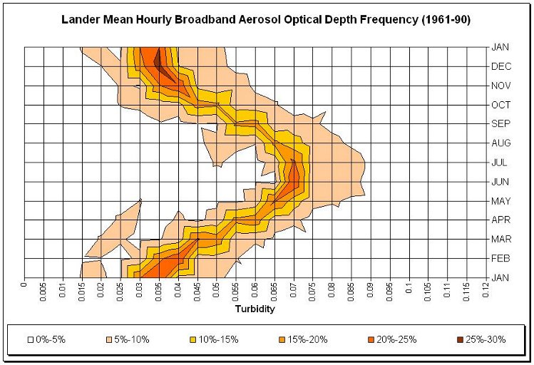
Figure 14.12. Same as Figure 14.8 except for Lander.

Figure 14.13

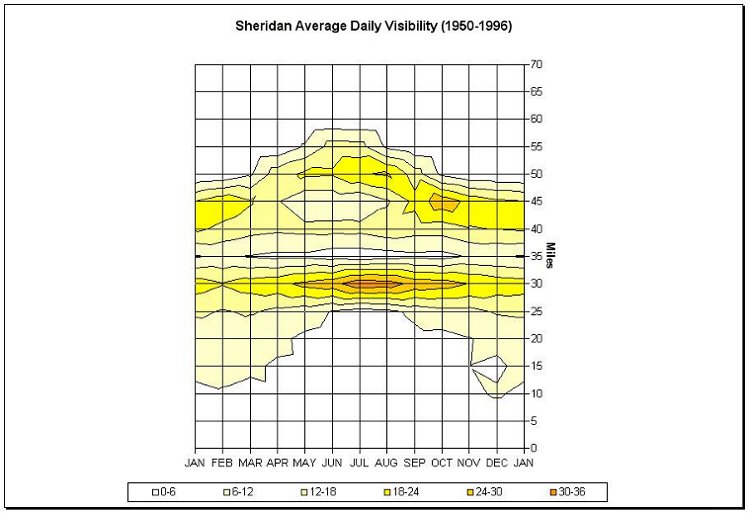
Figure 14.13. Same as Figure 14.7 except for Sheridan

Figure 14.14

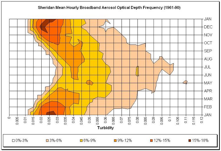
Figure 14.14. Same as Figure 14.8 except for Sheridan (note different scaling)

14.3.1 Atmospheric Aerosols¹¹⁵

Particles less than 100 microns in diameter are referred to as aerosol particles. These are aerodynamically stable and settle out slowly from the atmosphere. Smaller particles (approximately 1 micron) fall so slowly that they can take days or years to settle out of a quiescent atmosphere. For a turbulent atmosphere they may never fall out; however, they can be washed out by rain in a process called rainout or washout, leading to wet deposition onto the earth's surface.^115a

The mean number of days by month with obstruction to vision based on atmospheric aerosols for Casper, Lander, and Sheridan is summarized in Table 14.C. Fog, smoke, haze, blowing snow, dust, and sand are used in this compilation. Obstructions to vision are less frequent during mid-day and during the summer months, when temperature inversions are minimal.

Table 14.C. Average frequency (percent) by month with obstruction to vision
from aerosols for Casper (1950-1990), Lander and Sheridan (1948-1990).

	JAN	FEB	MAR	APR	MAY	JUN	JUL	AUG	SEP	OCT	NOV	DEC
CASPER	1.8	2.6	3.2	3.0	2.3	0.8	0.3	0.3	1.4	1.8	2.0	1.8
LANDER	1.5	1.4	0.6	0.7	0.6	0.2	0.1	0.1	0.5	0.7	1.6	1.4
SHERIDAN	2.4	2.3	2.8	1.8	0.7	0.6	0.2	0.2	1.1	1.0	2.2	2.3

14.3.2 Fog

The number of days with fog are quite low across the lower elevations of Wyoming. Cheyenne has the largest number of days with fog due in part to up-slope wind conditions when high pressure is situated to the north of the state. The summer rarely sees fog while the greatest frequency generally occurs in the spring. In Table 14.D., the monthly and annual number of days with reported fog is provided for the state's first order weather stations. Fog occurs quite often at higher elevations when mountains are embedded in clouds. Fog is essentially clouds that touch the ground. With radiational heating after sunrise, fog is known to burn-off. When air is completely saturated at 100 percent relative humidity, fog results. If this parcel of moist air is heated by the sun, through warm air advection, compressional heating, or vertical mixing with drier air aloft, the relative humidity drops and the fog dissipates.

Table 14.D. Monthly number of days with fog for Casper, Cheyenne, Lander, and Sheridan (1992-2002)

	JAN	FEB	MAR	APR	MAY	JUN	JUL	AUG	SEP	OCT	NOV	DEC	ANN
CASPER	1	1	1	1	1	*	*	*	1	1	1	1	9
CHEYENNE	1	2	3	3	3	2	1	1	2	2	2	1	24
LANDER	1	1	*	*	*	*	0	*	*	*	1	1	4
SHERIDAN	1	1	1	*	*	*	*	*	*	1	1	1	6

* denotes <0.5 days

14.3.3 Blowing Snow^115b

When the ground is completely snow covered, a motorist's visibility varies with wind speed in a predictable way (V=1.1 * 10⁸ / U₁₀⁵) where V is visibility in meters, and wind speed measured at 10 m (33 ft) (U₁₀) in meters per second. Visibility in blowing snow conditions is therefore approximately inversely proportional to the fifth power of wind speed. Because visibility is so sensitive to wind speed, fluctuations in wind speed makes driving in blowing snow hazardous. Over a period of 10 minutes, wind speed typically various 30 to 50 percent from the average, which causes extreme variations in visibility. For example, in Table 14.E, if wind speed averages 60 km/h (37 mph) with a variation of +/- 40 percent, visibility could vary from 1100 m (3609 ft) to 16 m (52 ft).

Table 14.E. Visibility vs 10 m wind speed for unlimited snow on the ground and without precipitation, assuming a 40 percent gust factor